
What is MS Excel?
Microsoft Excel is a spreadsheet program that allows us to store, organise and analyse information. Many people imagine that Excel is a tool only for specialists who process complicated data, but in reality anyone can learn to take advantage of Excel's powerful features. Whether we are keeping a household budget, organising a training log or creating an invoice, Excel makes it easy to work with many different kinds of data. Because it is part of the Microsoft Office family, it is used everywhere for accounts, marksheets, budgets, inventories and any work that involves rows and columns of data.
The real beauty of Excel lies in its ability to simplify these tasks. Working with a paper spreadsheet is complicated, time-consuming and limited. On paper, if a portion of our row data changes, we must erase and re-enter it, and then we must also erase and recalculate every derived figure — such as the totals or averages that were affected by that change. Excel removes all of this drudgery: it recalculates everything for us automatically the instant a number changes.
What can Excel do?
Excel can be used to make quick and easy financial analysis; to analyse data of every kind; to create presentations with charts (its graph utilities); to retrieve data from external data sources and use it inside our worksheets; to calculate using data from multiple worksheets at once; to create web pages with ease; and even to run queries on data available on the web. In short, it gathers the abilities of a calculator, a filing cabinet, a graphing tool and a small database into a single program.
- Calculate — add, subtract, multiply, divide and use hundreds of ready-made functions.
- Organise — sort, filter and group large lists, and search for data that meets a condition.
- Visualise — draw two-dimensional and three-dimensional column charts, pie charts and many other chart types.
- Analyse — summarise data with Pivot Tables and test outcomes with What-If tools.
Microsoft Excel is a full-featured spreadsheet program that allows us to organise data, complete calculations, make decisions, transform data into graphs, and develop professional-looking reports.
The three major parts of Excel
- Worksheets — worksheets let us enter, calculate, manipulate and analyse data such as numbers and text. This is the grid we type into.
- Charts — charts represent data pictorially. Excel can draw two-dimensional and three-dimensional column charts, pie charts and other types of chart.
- Databases — databases manage data. Once we enter data onto a worksheet, Excel can sort the data, search for specific data, and select only the data that meets certain criteria.
Key words to know
- A Workbook is the whole Excel file (extension .xlsx).
- A Worksheet (or sheet) is one page inside the workbook; a workbook can hold up to 255 sheets.
- A Cell is one box — the meeting point of a row and a column.
- One sheet has 10,48,576 rows and 16,384 columns (A–XFD).
Opening Excel (Start Menu)
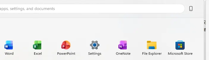
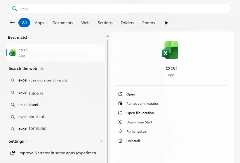
Before we can use Excel we have to open it. The traditional path is Start → All Programs → Microsoft Office → Microsoft Excel; if a shortcut already sits on the desktop we can instead simply double-click the desktop icon. On modern Windows the fastest way is through the Start menu search, shown below.
Step 1 Click the Start button at the bottom-left of the screen (the Windows logo). The Start menu opens. You can click Excel directly if you see its green icon in the pinned apps.
Step 2 If you don't see it, simply type “excel”. Windows searches and shows Excel as the Best match. Click it (or click Open) and Excel starts.
The Excel Start Screen
When we open Excel for the first time, the Excel Start Screen appears. From here we can do three things: create a new workbook, choose a template, or access our recently edited workbooks. The left side lists Recently Edited Workbooks for one-click reopening, while the right side shows a New Workbook tile and a row of ready-made Templates. To reach the normal Excel grid, locate and select Blank workbook.
The Excel Window & Backstage
If we have previously used an earlier version of Excel, this environment will feel very familiar. It continues to use features like the Ribbon and the Quick Access Toolbar, where we find the commands to perform common tasks, as well as the new full-screen Backstage view. When Excel opens we see the worksheet grid with the Ribbon of tools on top. It is worth learning every part below, because every later task uses them.
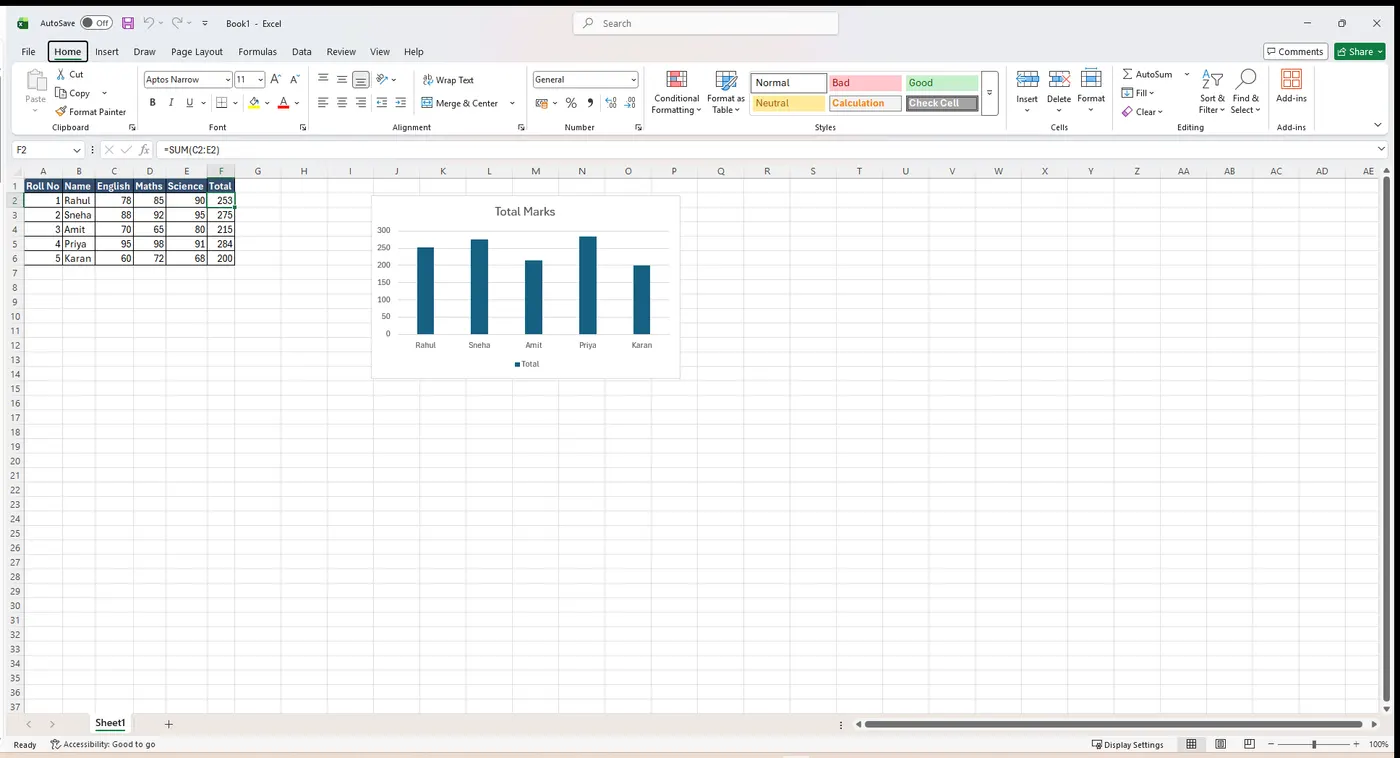
The Ribbon: Excel uses a tabbed Ribbon system instead of the traditional menus of older programs. The Ribbon contains multiple tabs (Home, Insert, Page Layout, Formulas, Data, Review, View), and each tab is divided into several groups of related commands. We use these tabs to carry out the most common tasks in Excel.
The Quick Access Toolbar (QAT): located just above the Ribbon, the Quick Access Toolbar lets us reach common commands no matter which tab is currently selected. By default it includes the Save, Undo and Repeat (Redo) commands, and we can add other commands to it depending on our preference.
- Title Bar — shows the workbook name at the very top of the window.
- File Menu (File tab) — the green tab that opens Backstage view.
- Name Box — shows the address of the selected (active) cell, e.g. A1.
- Formula Bar — shows, and lets us edit, the content or formula of the active cell.
- Cell — the single highlighted box we are working in.
- Work Area — the grid of cells where we type our data.
- Status Bar — the bottom strip; it shows the Average, Count and Sum of the selected cells.
- View Options / Views option — buttons (Normal, Page Layout, Page Break Preview) to switch how the sheet is shown.
- Help — the ? icon that opens Excel's help window (covered later).
Help
The Help icon can be used to get Excel-related help any time we need it. Clicking on the ? opens the Excel Help window, where we have a list of common topics to browse. We can also search for a specific topic using the search bar at the top.
Zoom options
The zoom control at the bottom-right lets us zoom in for a closer look at our text. It consists of a slider that we can drag left or right to zoom in or out, and we can also click the − and + buttons to decrease or increase the zoom factor. The maximum zoom supported by Excel is 500% and the minimum is 10%, while 100% is indicated by the mark in the middle. (Zoom only changes the on-screen size, not the printed size, and the Zoom option is also available on the View tab.)
Workbooks: New, Open, Save & Templates
Excel files are called workbooks. Whenever we start a new project in Excel we need to create a new workbook. There are several ways to begin: we can create a brand-new workbook — either a blank one or one based on a pre-designed template — or we can open a workbook that already exists.
Create a new, blank workbook
Step 1 Select the File tab. The Backstage view will appear.
Step 2 Select New and then click Blank workbook (or simply press Ctrl + N).
Step 3 A new, blank workbook appears, ready for typing.
Open an existing workbook
Step 1 Navigate to Backstage view and then click Open (or press Ctrl + O).
Step 2 Select a location option. Open Recent Workbooks displays all of the workbooks we have recently edited, for one-click access; otherwise browse to the file.
Using templates
To save typing, we can start from a ready-made template (calendar, budget, invoice and many more) instead of a blank sheet.
Step 1 In Backstage view, select New. Several templates appear below the Blank workbook option.
Step 2 Select a template to review it.
Step 3 A preview of the template appears, along with additional information about how the template can be used.
Step 4 Click Create to use the selected template.
Saving, Sharing & Exporting Workbooks
Saving and sharing
Whenever we create a new workbook, we need to know how to save it so that we can access and edit it later. As in previous versions of Excel, we can save files locally to our computer. But, unlike older versions, Excel also lets us save a workbook to the cloud using SkyDrive. We can also export and share workbooks with others directly from inside Excel.
Save and Save As
Excel offers two ways to save a file — Save and Save As. They work in similar ways but with a few important differences:
- Save (Ctrl + S) — when we create or edit a workbook we use the Save command to store our changes; this is the command we use most of the time. The first time we save a file we need to choose a file name and a location; after that, clicking Save simply stores it again under the same name and location.
- Save As (F12) — we use this command to create a copy of a workbook while keeping the original. With Save As we must choose a different name and/or a different location for the copied version.
Compatibility Mode
Sometimes we need to work with workbooks that were created in an earlier version of Excel, such as older versions of Excel. When we open these older workbooks they appear in Compatibility mode. Compatibility mode disables certain newer features, so we will only be able to use the commands found in the program that originally created the workbook. For example, if we open a workbook created in an older version of Excel, we can use only the tabs and commands that were available in that version.
Exporting workbooks
By default, Excel workbooks are saved in the .xlsx file type. However, there may be times when we need another file type, such as a PDF or an Excel 97-2003 workbook. It is easy to export our workbook from Excel into a variety of file types.
Export as a PDF file
Exporting our workbook as an Adobe Acrobat Document — commonly known as a PDF — is especially useful when sharing with someone who does not have Excel; a PDF lets recipients view but not edit the content.
Step 1 Click the File tab to access Backstage view.
Step 2 Click Export and then select Create PDF/XPS.
Step 3 The Save As dialog box appears; select the location where we wish to export the workbook, enter a file name, and click Publish.
Export in other file types
We may also export the workbook in other types — for example an Excel 97-2003 workbook to share with people using an older version, or a .CSV file if we need a plain-text version.
Step 1 Click the File tab to access Backstage view.
Step 2 Click Export and then select Change File Type.
Step 3 Select a common file type and then click Save As.
Step 4 The Save As dialog box appears; select the location, enter a file name, and click Save.
Cells, Rows & Columns
Whenever we work with Excel we enter information, or content, into cells. Cells are the basic building blocks of a worksheet. Every worksheet is made up of thousands of rectangles, and each of these rectangles is called a cell. A cell is the intersection of a row and a column.
- Columns run up–down and are identified by letters (A, B, C …).
- Rows run left–right and are identified by numbers (1, 2, 3 …).
- Every cell has its own name, called its cell address or cell reference, based on its column and row. If the selected cell intersects column C and row 5, its cell address is C5. This address also appears in the Name Box.
Cell range
We can also select several cells at the same time. A group of cells is known as a cell range. Rather than using a single cell address, we refer to a range using the addresses of the first and last cells, separated by a colon. For example, a range that includes cells A1, A2, A3, A4 and A5 is written as A1:A5.
Selecting
- One cell — click it. The selected single cell is called the active cell and is recognised by a black border around it.
- A whole column — click its letter heading.
- A whole row — click its number heading.
- A range with the keyboard — hold Shift and press the arrow keys.
- Everything — click the Select All box at the top-left corner of the grid (or press Ctrl + A).
Entering & clearing data
Click a cell, type, and press Enter. Any text we enter is aligned to the bottom-left of the cell, while any number is aligned to the bottom-right. To erase only the contents but keep the formatting, use Home → Editing → Clear → Clear Contents (or press Delete).
Modifying Columns, Rows & Cells
By default, every row and column of a new workbook is set to the same height and width. Excel allows us to modify column width and row height in a variety of ways — including, as we shall see, wrapping text and merging cells. When the content of a column or row cannot be fully displayed, we can make all of it visible by changing the size.
Modifying column width by dragging
Step 1 Position the mouse over the column line in the column heading so that the white cross becomes a double arrow.
Step 2 Click, hold and drag the mouse to increase or decrease the column width.
Step 3 Release the mouse; the column width is changed. (The same three steps, applied to a row line, change the row height.)
AutoFit column width
The AutoFit feature sets a column's width to fit its content automatically.
Step 1 Position the mouse over the column line so the white cross becomes a double arrow.
Step 2 Double-click the mouse; the column width changes automatically to fit the content.
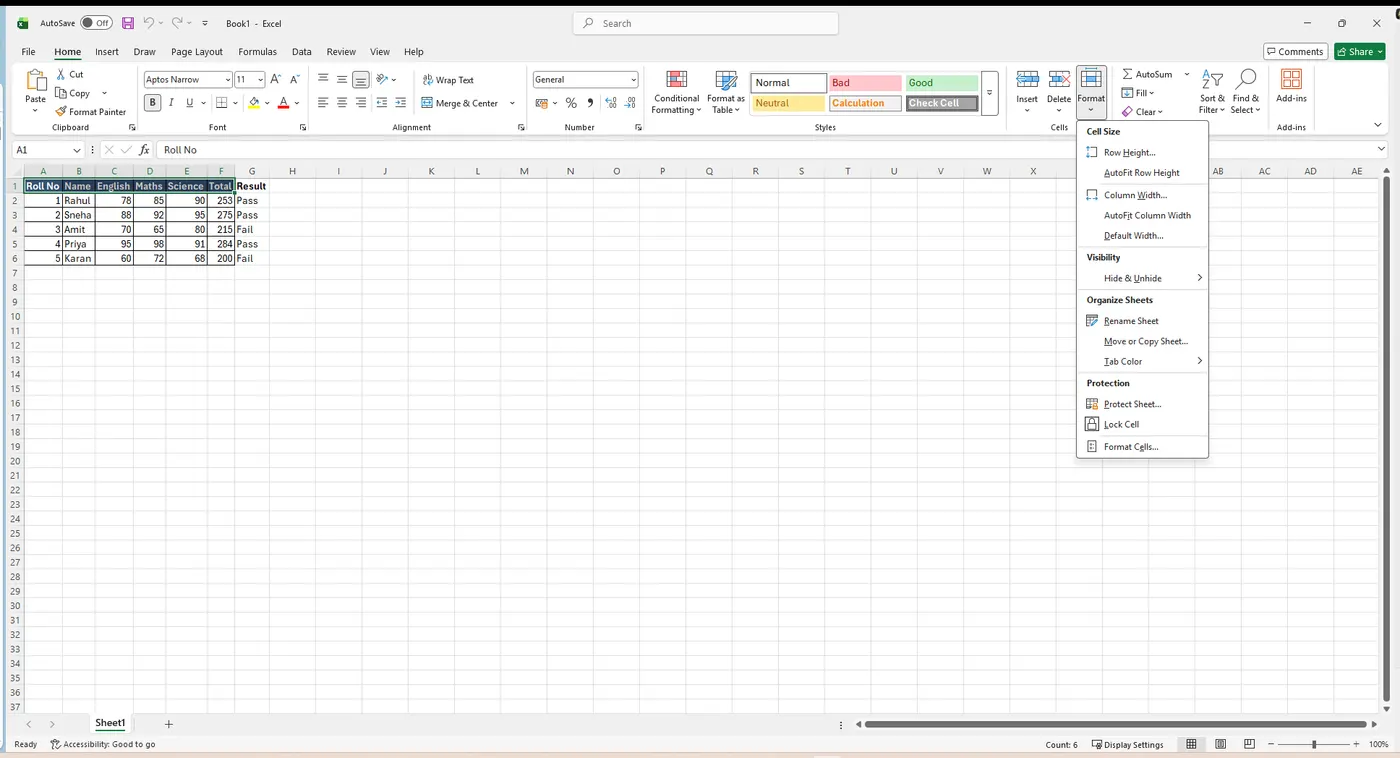
We can also AutoFit several columns at once: select the columns we want, then choose AutoFit Column Width from the Format drop-down menu on the Home tab (Home → Cells → Format). The same Format menu also offers AutoFit Row Height.
Step Open Home → Format and choose AutoFit Column Width.
Resize ALL rows or columns at once
Rather than resizing rows and columns individually, we can modify the height and width of every row and column at the same time, giving the whole worksheet a uniform size. (1) Locate and click the Select All button to select every cell in the worksheet. (2) Position the mouse over a row line so the white cross becomes a double arrow. (3) Click, hold and drag to increase or decrease the row height. (4) Release the mouse when satisfied with the new size — every row (or column) takes the same new size.
Insert, Delete, Move & Hide
After we have been working with a workbook for a while, we may find that we want to insert new columns or rows, delete certain ones, move them to a different location, or even hide them. Each of these is a simple right-click operation.
Inserting rows
Step 1 Select a row by clicking its number, then right-click the mouse button.
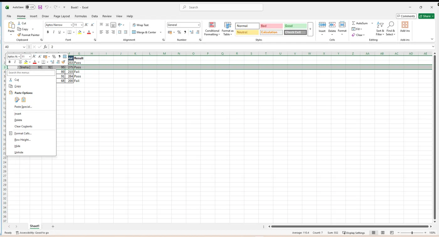
Step 2 Select the Insert option.
Step 3 The new row appears above the selected row.
Inserting columns
First select the column heading to the right of where the new column should appear — for example, to insert a column between columns D and E, select column E. (1) Right-click the selected column. (2) Select Insert. (3) The new column appears to the left of the selected column.
Delete
Right-click the row number or column letter and choose Delete (the Delete Sheet command, by contrast, lives on the Home tab in the Cells group).
Move a row or column
Sometimes we want to move a column or row to rearrange the content of the worksheet. (1) Select the desired column or row, then click Cut on the Home tab or press Ctrl + X. (2) Click the Insert command on the Home tab and select Insert Cut Cells from the drop-down menu. (3) The column is moved to the selected location and the columns to the right shift right.
Hide & Unhide
At times we may want to compare certain rows or columns without changing the organisation of the worksheet. (1) Select the row or column(s) to hide, right-click, and choose Hide from the formatting menu. (2) The columns are hidden, and a thin green row or column line indicates the location of the hidden data. (3) To unhide, select the columns to the left and right of the hidden columns — in other words, the columns on both sides. (4) Right-click and choose Unhide; the hidden columns reappear.
Wrapping Text & Merging Cells
Whenever we have too much cell content to be displayed in a single cell, we may decide to wrap the text or merge the cell rather than resizing a column. Wrapping the text automatically modifies the cell's row height, allowing the contents to be displayed on multiple lines. Merging lets us combine a cell with adjacent, empty cells to create one large cell.
Wrapping text in cells
(a) Select the cells we wish to wrap — for example, the cells in column C. (b) Select the Wrap Text command on the Home tab. (c) The text in the selected cells is wrapped onto multiple lines and the row grows taller. (d) Click Wrap Text again to unwrap the text. (Compare: the column before text wrapping vs. the column after text wrapping.)
Merging cells with Merge & Center
Merging joins several cells into one big cell — useful, for example, for a title across the top of a table. (a) Select the cell range we want to merge together, for example D1:H1. (b) Select the Merge & Center command on the Home tab. (c) The selected cells are merged into one and the text is centred. (Compare: the cells before vs. the cells after the merge.)
Step Select the cells, then click the arrow next to Merge & Center to pick a merge option.
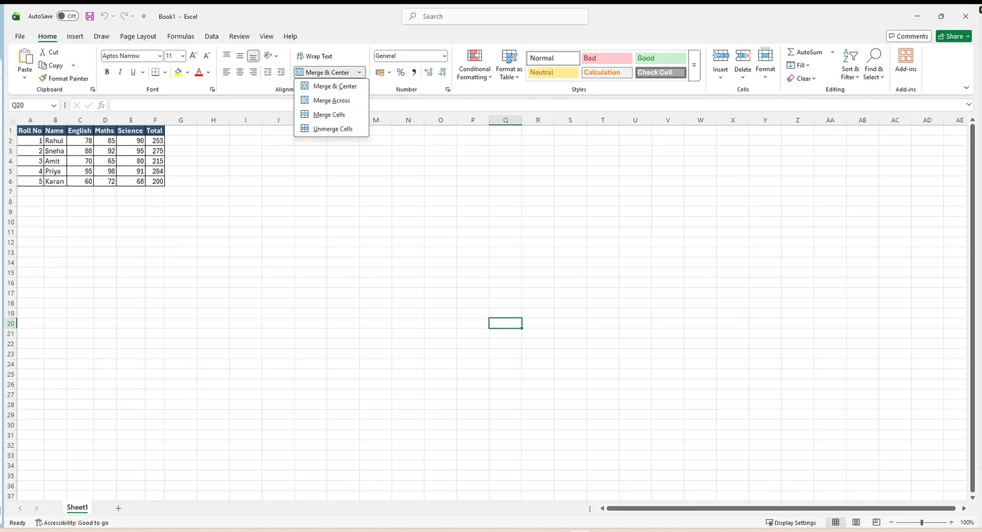
- Merge & Center — join the cells into one and centre the text.
- Merge Across — merge each row separately (good for multi-row selections).
- Merge Cells — join into one cell but do not centre.
- Unmerge Cells — split a merged cell back into separate cells.
Formatting Cells — Font & Alignment
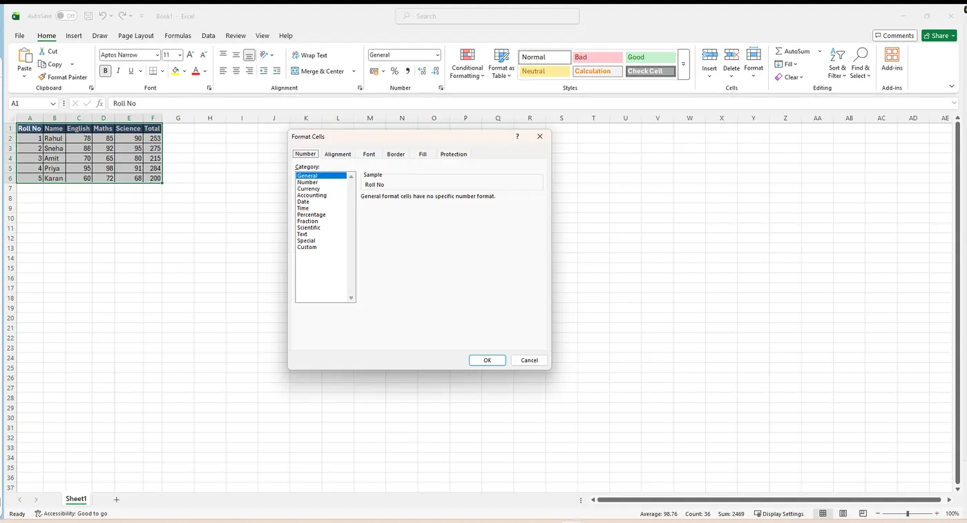
By default, all cell content uses the same formatting, which can make a workbook full of information difficult to read. Formatting lets us customise the look and feel of the workbook, draw attention to specific sections, and make the content easier to view and understand. All of it lives on the Home tab, and the full set of options is in the Format Cells dialog (Ctrl + 1).
Changing the font, size and style
By default, the font of each new workbook is set to Calibri at font size 11; however, Excel provides a wide variety of other fonts. To customise our cell text, select a cell and click the drop-down arrow next to the Font command on the Home tab to open the Font menu. As we move the mouse over the different options, a live preview shows how the text will look, and clicking applies the chosen font and size. For emphasis, use the B (Bold), I (Italic) and U (Underline) buttons — or press Ctrl + B for bold, Ctrl + I for italics, and Ctrl + U for underline — after selecting the cell(s) we wish to modify.
Text alignment
By default, any text entered into the worksheet is aligned to the bottom-left of a cell, and any numbers are aligned to the bottom-right. Changing the alignment of cell content lets us choose how the content is displayed in a cell, which can make it easier to read. MS Excel has two types of alignment:
- Horizontal alignment — we can align the cell text Left, Center, Right or Justify.
- Vertical alignment — we can align the cell text Top, Middle or Bottom.
We can also rotate text within a cell using the Text Orientation option.
Step Select the cells and press Ctrl + 1 to open Format Cells, where Number, Alignment, Font, Border, Fill and Protection all sit on separate tabs.
Borders, Fill & Number Formats
Cell borders & fill colours
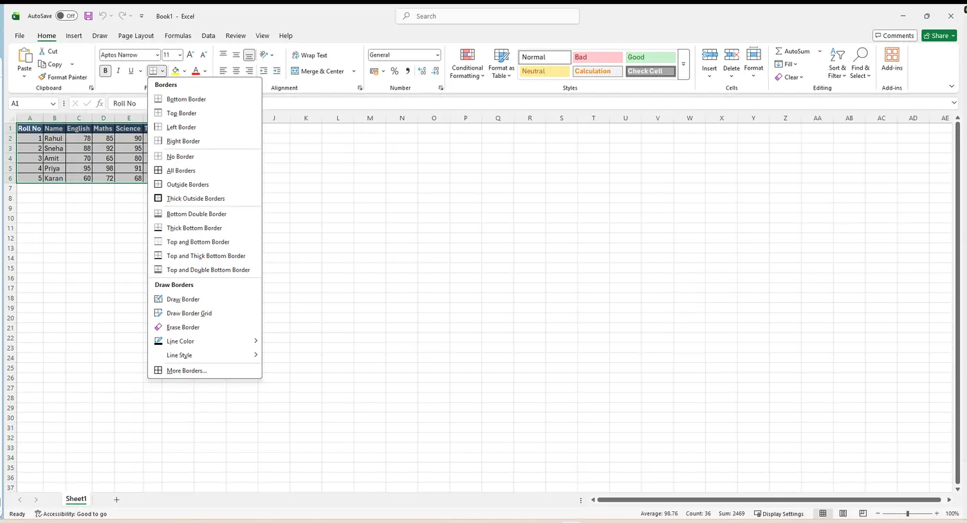
Cell borders and fill colours allow us to create clear, defined boundaries for the different sections of our worksheet. Both commands are in the Font group on the Home tab. Open the Borders menu to pick a border style, change the line style, and change the colour of the borders using the Draw Borders tools at the bottom of the Borders drop-down menu; use the Fill Color bucket to shade the selected cells.
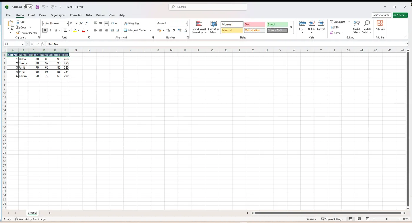
Formatting text and numbers
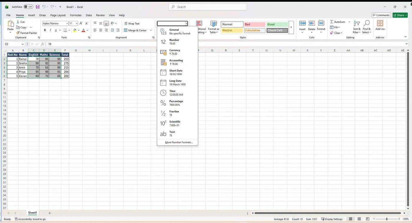
One of the most powerful tools in Excel is the ability to apply specific formatting for text and numbers. Instead of displaying all cell content in exactly the same way, we can use formatting to change the appearance of dates, times, decimals, percentages (%), currency ($) and much more. The Number group lets us show the same underlying value in these different ways — open the Number Format list to choose.
Step Select the cells and pick a format from the Number Format list (Home tab).
Worksheet Basics
Every workbook contains at least one worksheet by default. When working with a large amount of data, we can create multiple worksheets to help organise the workbook and make it easier to find content. The sheet tabs sit just below the work area. We can add a new worksheet, rename a worksheet, make a copy of one, move one, and delete one. To add a new worksheet to the workbook, press the + button near Sheet1.
- Add — click the + button next to the last sheet tab.
- Rename — double-click the tab and type a new name.
- Copy / Move — right-click the tab and choose Move or Copy.
- Delete — right-click the tab and choose Delete.
- Tab colour — right-click → Tab Color to colour-code sheets.
- Protect Sheet — right-click → Protect Sheet to stop others editing or deleting it.
Grouping worksheets
We can work with each worksheet individually, or we can work with multiple worksheets at the same time by combining them into a group. Any change made to one worksheet in a group is made to every worksheet in that group. To group sheets: (a) select the first worksheet to include; (b) press and hold the Ctrl key; (c) select each additional worksheet we want in the group, continuing until all the desired worksheets are selected; (d) release the Ctrl key — the worksheets are now grouped. While grouped, we can navigate to any worksheet in the group, and any change we make will appear on every worksheet in it. However, if we select a worksheet that is not in the group, all of the worksheets become ungrouped.
Page Layout
The commands on the Page Layout tab let us control the way our content appears on a printed page, including the page orientation, margin size and more. Other options, such as print titles and page breaks, help make a workbook easier to read.
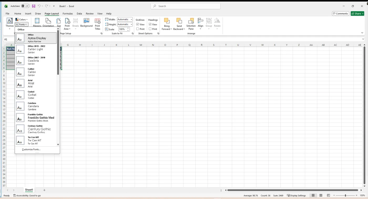
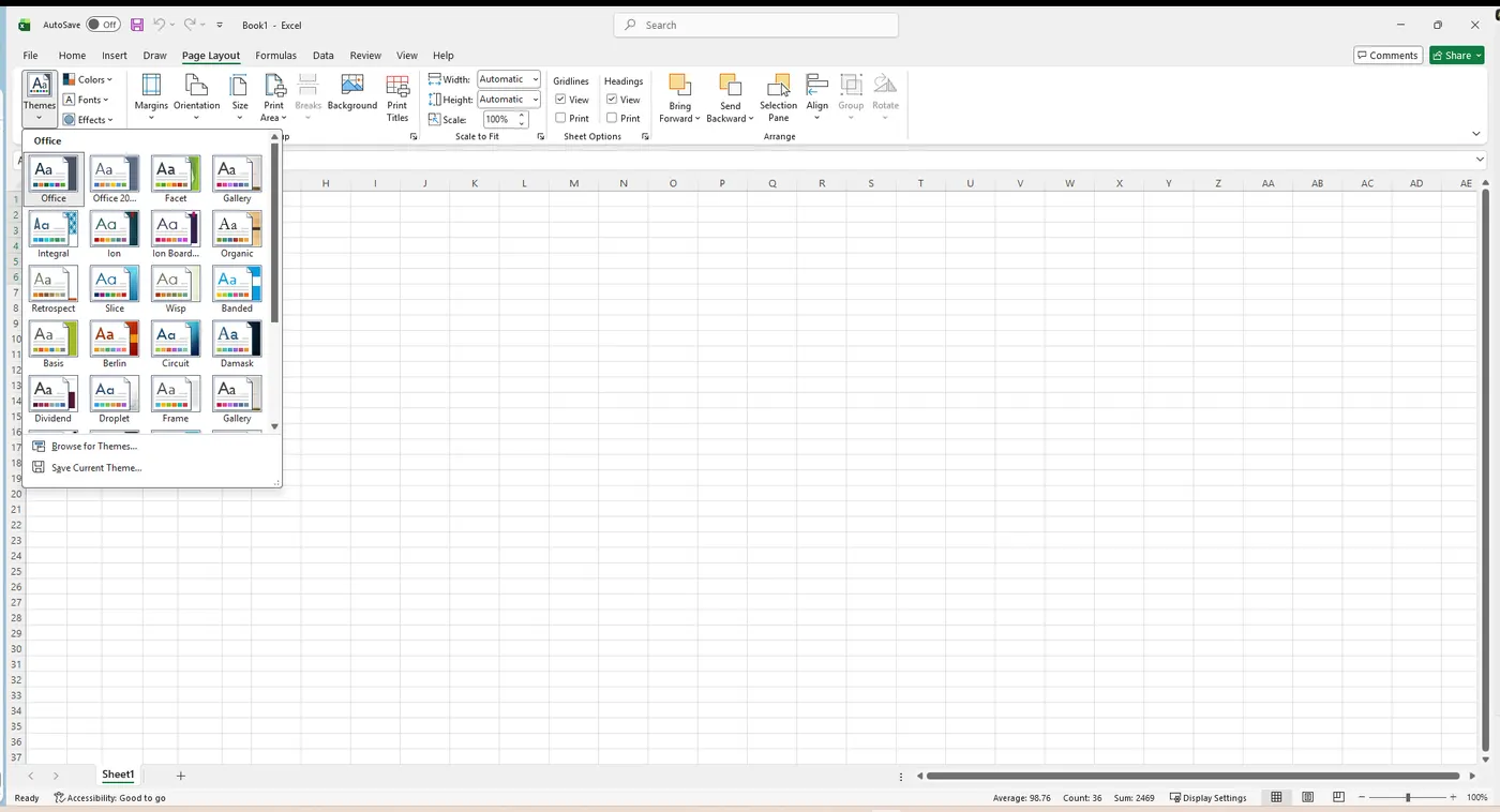
- Page Orientation — Excel offers two orientation options. Landscape orients the page horizontally (wide), while Portrait orients it vertically (tall).
- Formatting Page Margins — a margin is the space between the content and the edge of the page. By default every workbook's margins are set to Normal, a one-inch space between the content and each edge. Sometimes we adjust the margins so the data fits more comfortably; Excel includes a wide variety of pre-defined margin sizes.
- Including Print Titles — if our worksheet uses title headings, it is important to include those headings on every printed page; a printed workbook would be extremely difficult to read if the headings appeared only on the first page. The Print Titles command lets us select specific rows and columns to appear on each page.
- Inserting a Page Break — to print different parts of the workbook on separate pages, we can insert a page break. There are two types: vertical page breaks separate columns, while horizontal page breaks separate rows. Page breaks are viewed in Page Break Preview.
- Inserting Headers & Footers — we can make the workbook easier to read and more professional by including headers and footers. The header is a section that appears in the top margin, while the footer appears in the bottom margin (page number, title, date).
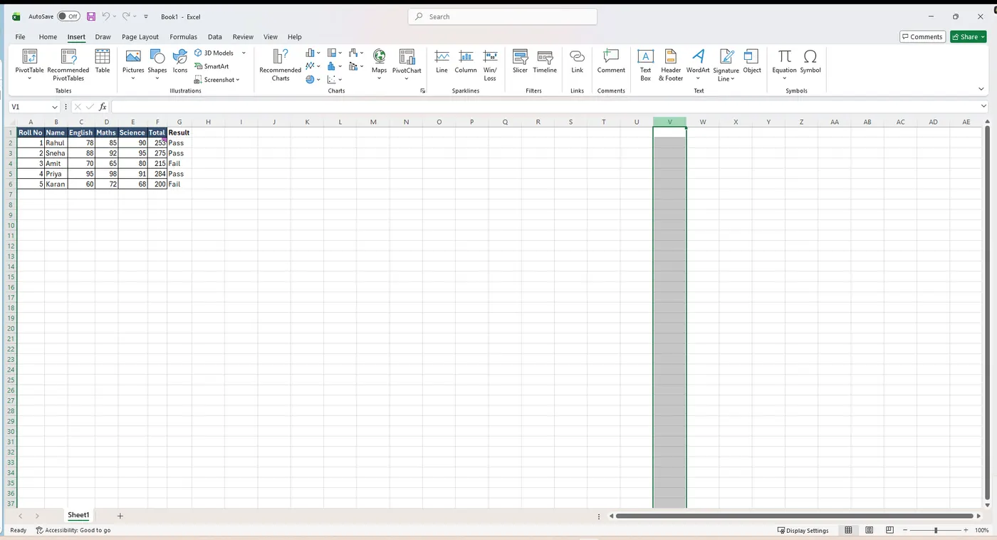
Headers & Footers Insert → Header & Footer switches to Page Layout view where you can type into the top and bottom margins.
Printing a Workbook
Before printing an Excel workbook, it is important to decide exactly what information we want to print. For example, if we have multiple worksheets in the workbook, we must decide whether to print the entire workbook or only the active worksheets. There may also be times when we want to print only a selection of content. A printed copy of a file is also called a hard copy. Press Ctrl + P (or File → Print) to open the Print screen: on the right we see a live preview of exactly what will print, and on the left are all the settings.
Step Choose the printer, how many copies, and what to print, then click Print.
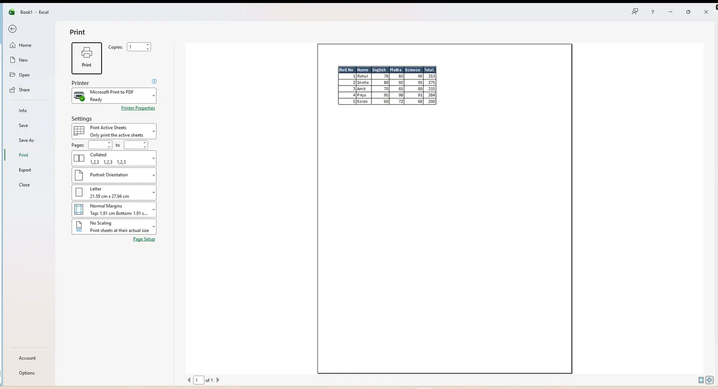
- Print Active Sheets — print the open sheet, the Entire Workbook, or just the Selection you highlighted.
- Copies — how many to print; Collated keeps each copy in page order.
- Orientation, paper size and margins can also be changed here before printing.
Formulas & the AutoSum
One of the most powerful features in Excel is the ability to calculate numerical information using formulas. Just like a calculator, Excel can add, subtract, multiply and divide. A formula is an instruction to perform a calculation, and a standard formula always begins with an equals sign (=).
Mathematical operators
Each formula uses mathematical operators: a plus sign for addition (+), a minus sign for subtraction (−), an asterisk for multiplication (*), a forward slash for division (/), and a caret (^) for exponents. For example =2+2 or =5*5. (Note that we cannot use spaces while typing a formula in a cell.)
Use cell references, not just numbers
We can create simple formulas manually (for example =2+2 or =5*5), but most of the time we use cell addresses to build a formula — this is known as making a cell reference. Instead of =78+85, write =C2+D2. Using cell references ensures our formulas are always accurate, because we can change the value of a referenced cell without having to rewrite the formula. By combining a mathematical operator with cell references we can create a variety of simple formulas, and formulas can also include a combination of cell references and numbers.
Point-and-click & the fill handle
Rather than typing cell addresses manually, we can point and click on the cells we wish to include while building a formula; this can save a lot of time and effort. To repeat a formula across adjacent cells, drag the small square at the bottom-right of the cell — the fill handle — and Excel copies the formula, adjusting the references automatically, which saves a lot of effort when the same calculation is needed many times.
Creating complex formulas (order of operations)
Excel follows the standard order of operations. For example, it first adds the values inside the parentheses: (44.85 + 39.90) = $84.75; then it multiplies that value by the tax rate: $84.75 × 0.075; and the result shows that the sales tax is $6.36. It is especially important to enter complex formulas with the correct order of operations — otherwise Excel will not calculate the results accurately.
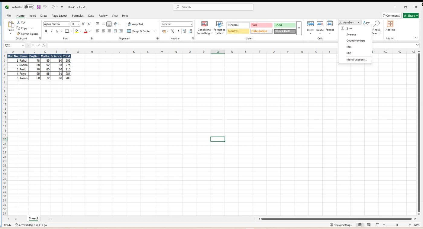
AutoSum Select the cell below a column of numbers and click AutoSum (Home or Formulas tab). Excel writes =SUM(…) for you. The dropdown also offers Average, Count, Max and Min.
Functions & the Function Library
A function is a ready-made, built-in formula available in Excel. We give it a range of cells — the argument — and it returns an answer. Excel has a wide variety of functions; here are some of the most common ones we use:
| Function | What it does | Example |
|---|---|---|
| SUM | adds all the values of the cells in the argument | =SUM(C2:C6) |
| AVERAGE | calculates the sum of the cells and divides by the number of cells | =AVERAGE(C2:C6) |
| COUNT | counts the number of cells with numerical data (handy for counting items in a range) | =COUNT(C2:C6) |
| MAX | determines the highest cell value in the argument | =MAX(C2:C6) |
| MIN | determines the lowest cell value in the argument | =MIN(C2:C6) |
Insert Function Press Shift + F3 (or click fx beside the formula bar) to search for any function and fill in its parts with help.
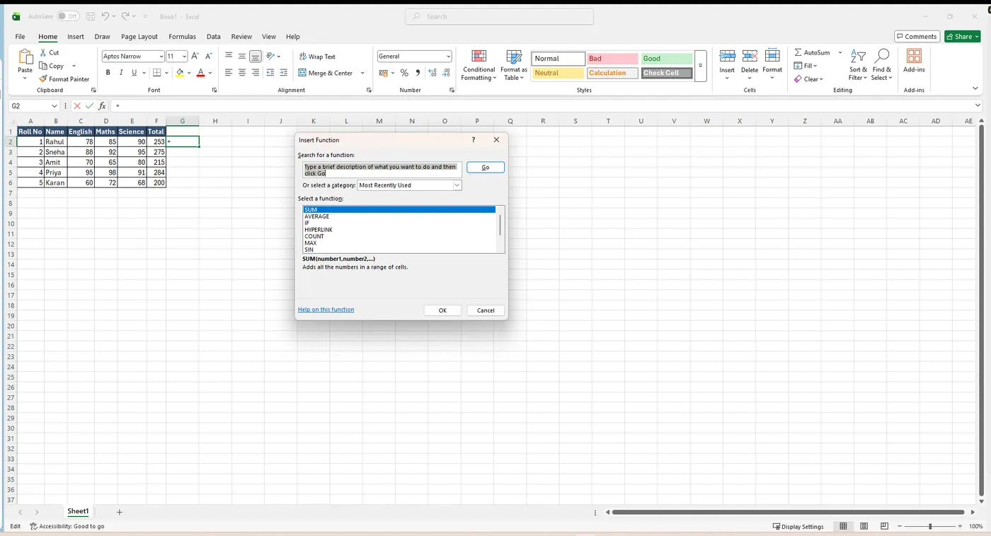
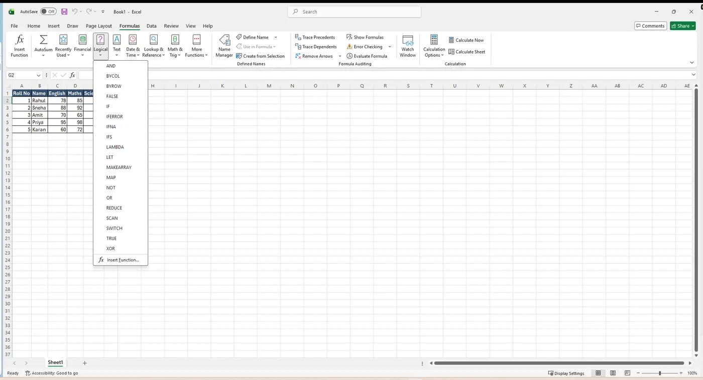
While there are hundreds of different functions in Excel, the ones we use most frequently depend on the kind of data our workbook contains. There is no need to learn every single function, but exploring the different types is helpful as we create new projects. The Formulas → Function Library lets us search for functions by category — Financial, Logical, Text, Date & Time, Lookup and much more — so we can browse instead of memorising. (Common date/time examples include =TODAY() for the current date and =NOW() for the current system time; =UPPER() converts text to capitals; =ROUND() rounds a number to a specific number of digits; and DB is an example of a financial function.)
Cell References & Formula Errors
Relative, Absolute & Mixed references (beyond the basics)
- Relative (C2) — when copied, it shifts (C2 → C3 → C4). This is the default.
- Absolute ($C$2) — the $ locks it so it never changes when copied.
- Mixed ($C2 or C$2) — locks only the column or only the row.
Order of operations
Excel calculates like maths: brackets first, then powers, then × and ÷, then + and −. So =(2+3)*4 gives 20, not 14. Use brackets to be sure.
Formula error messages
If Excel cannot calculate a formula it shows an error starting with #:
| Error | Meaning |
|---|---|
| #DIV/0! | trying to divide by zero |
| #N/A | a value is not available |
| #NAME? | Excel does not recognise the name/text used |
| #NULL! | an invalid intersection of two ranges |
| #NUM! | a number is used incorrectly |
| #REF! | refers to a cell that no longer exists |
| #VALUE! | wrong type of argument (e.g. text where a number is needed) |
| ##### | not an error — the column is just too narrow |
The IF Function (Conditional Formula)
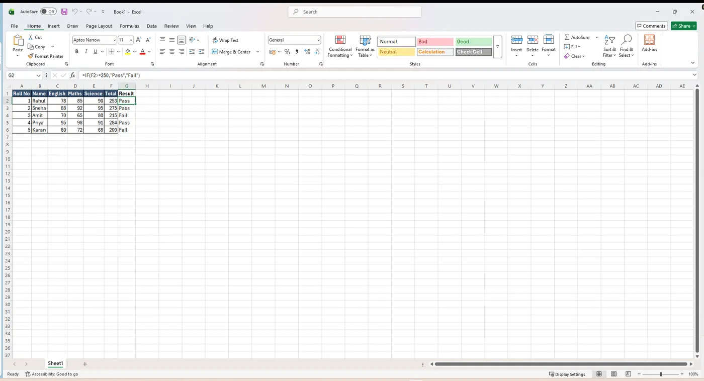
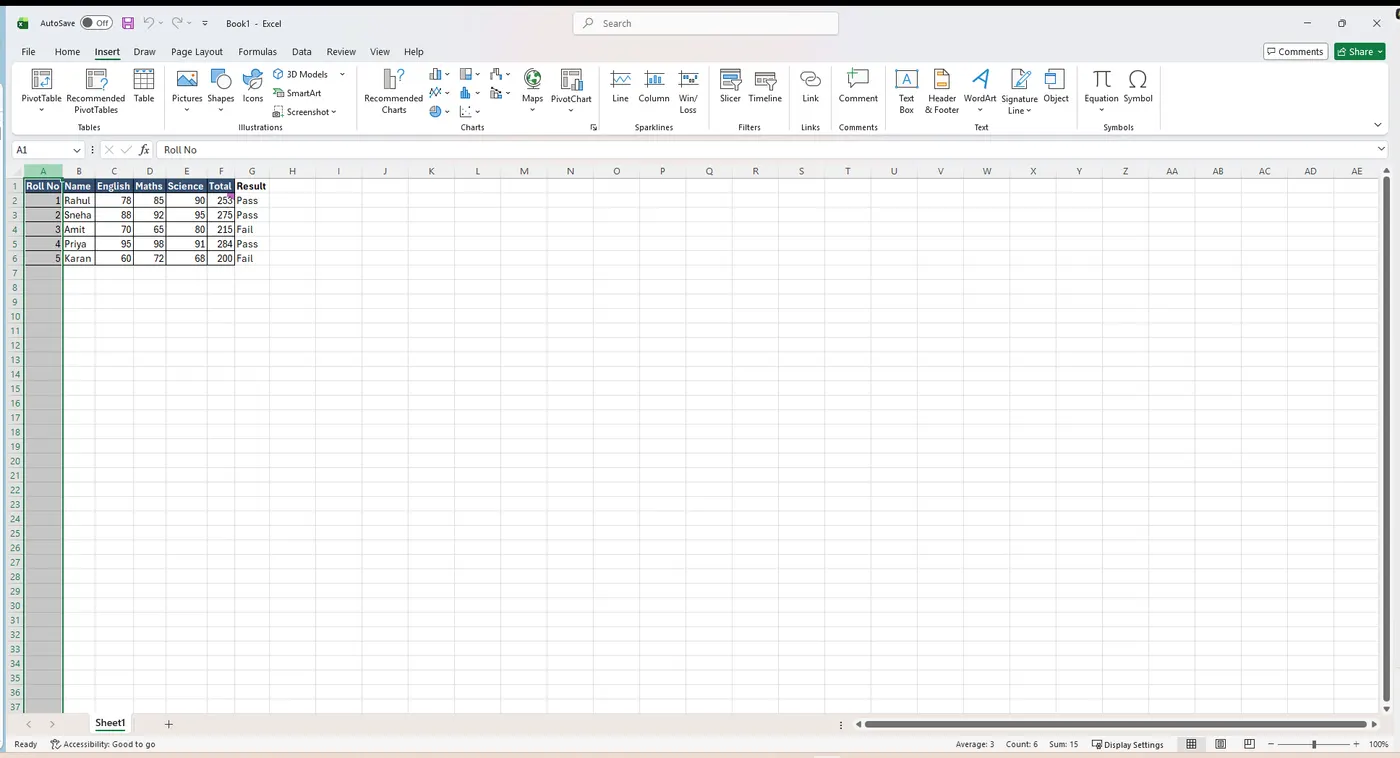
The IF function is one of the most useful functions available in Excel. When we design an IF function, we ask Excel to perform a test, and then tell Excel what to do if the result of the test is positive (true) or negative (false). Although it may look intimidating at first, it really is quite simple. (IF is a logical function.)
=IF(logical_test, value_if_true, value_if_false)
Consider a worked example: assume we enter the formula in cell D16 as =IF(A16=1, Faculty, Staff). The syntax breaks down as follows:
- =IF — every formula in Excel starts with the equals (=) sign, and the IF tells Excel to perform the IF function; the remaining information is inserted within parentheses.
- logical_test — any value or expression that results in True (1) or False (0). It asks Excel to test something; here Excel looks at cell A16 and determines whether its value equals 1.
- value_if_true — the value returned if the logical test is true. For instance, if A16 has a value of 1, Excel inserts the text “Faculty” in cell D16.
- value_if_false — the value returned if the logical test is false. For instance, if A16 has any value other than 1, Excel inserts the text “Staff” in cell D16.
The value_if_true and value_if_false parts of the function can each contain either text or formulas.
Example =IF(F2>=250,"Pass","Fail") — if the total in F2 is 250 or more it writes “Pass”, otherwise “Fail”.
Freeze Panes & Split
Whenever we work with a lot of data, it can be difficult to compare information in the workbook. Excel includes several tools that make it easier to view content from different parts of the workbook at the same time — chiefly the ability to freeze panes and split the worksheet.
Freezing rows & columns
We often want to see certain rows or columns all the time, especially header cells. By freezing rows or columns in place, we can scroll through our content while continuing to view the frozen cells. To freeze: (i) select the row or column we wish to freeze; (ii) click the View tab on the Ribbon; (iii) select the Freeze Panes command and then choose Freeze Panes from the drop-down menu; (iv) the rows are frozen in place, as indicated by a grey line, and we can scroll down while continuing to view the frozen rows at the top.
Step Select the row/column, then View → Freeze Panes and pick an option.
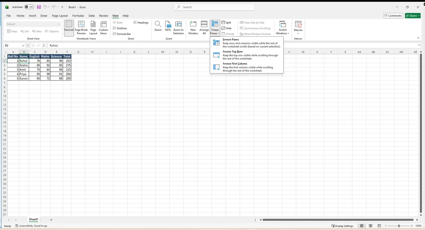
To unfreeze the rows or columns that have been frozen, go to the View menu and select the Unfreeze Panes option from the Freeze Panes command.
Splitting the worksheet
If the workbook contains a lot of content, it can be difficult to compare different sections. Besides opening a new window, Excel lets us split a worksheet into separate panes. The Split command divides the worksheet into multiple panes that scroll separately. To split: (i) select the cell where we wish to split the worksheet (in our example, cell D2); (ii) click the View tab and then select the Split command; (iii) the workbook is split into different panes, and we can scroll through each pane separately using the scroll bars to compare different sections. Click Split again to remove it.
Sorting & Filtering
Sorting
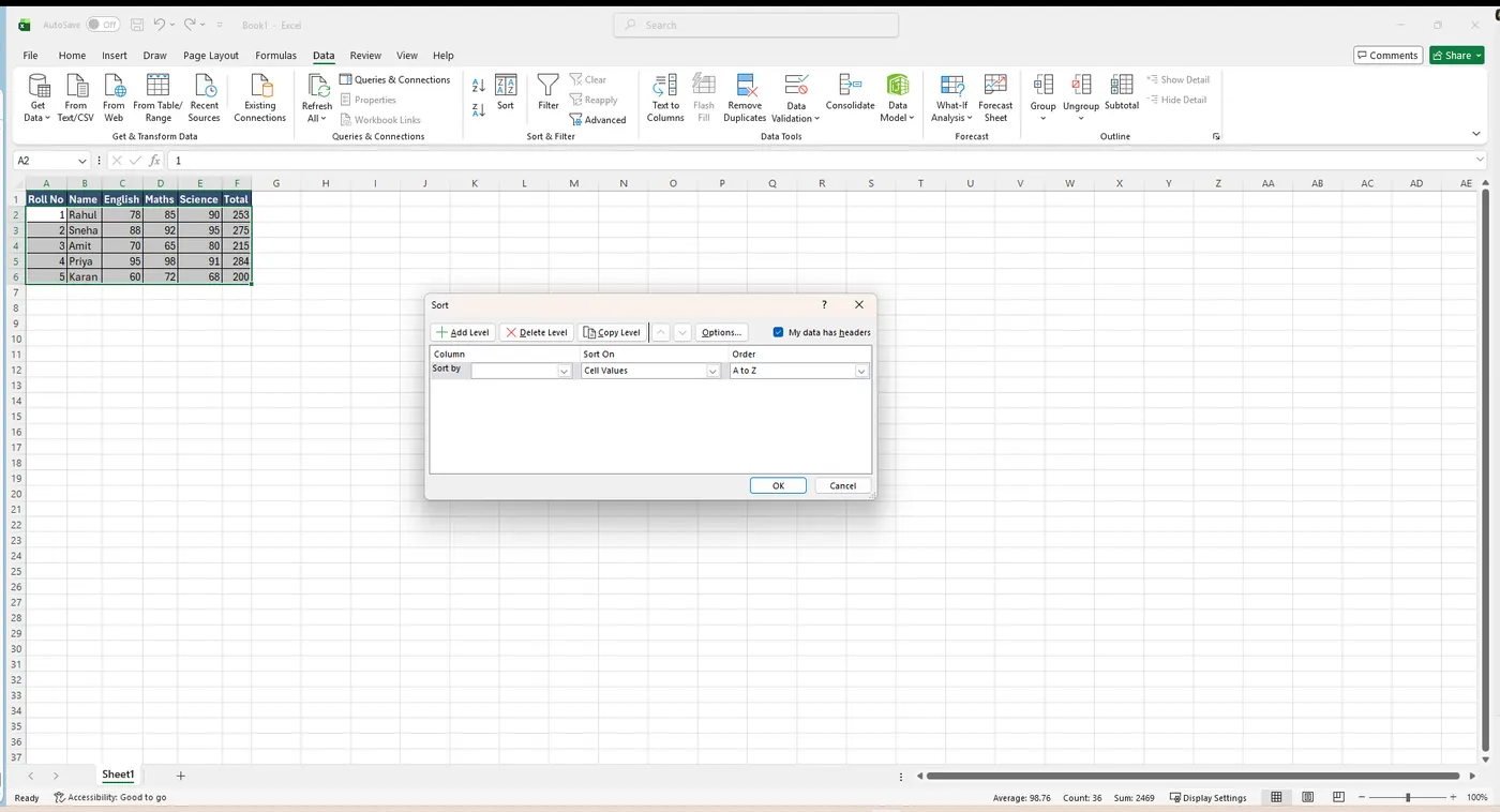
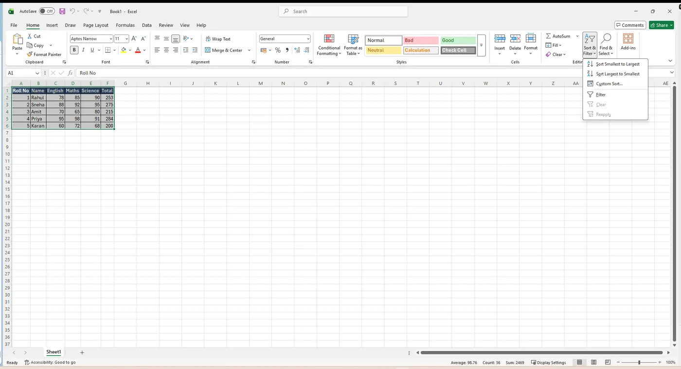
As we add more content to a worksheet, organising that information becomes especially important. We can quickly reorganise a worksheet by sorting our data — for example, organising a list of contacts by last name. Content can be sorted alphabetically, numerically and in many other ways. To sort: (a) select a cell range, or the rows or columns we wish to sort by; (b) select the Data tab and then click the A→Z command to sort A to Z (ascending), or the Z→A command to sort Z to A (descending); (c) the worksheet is sorted by the selected column. The two types of sorting in Excel are therefore Ascending and Descending. For more control, click Sort to open the Sort dialog and sort by several columns at once.
Step Data → Sort opens the dialog where you choose the column, what to sort on, and the order.
Filtering
Filters can be used to narrow down the data in our worksheet, so we view only the information we need. For filtering to work correctly, the worksheet should include a header row that identifies the name of each column. To filter: (a) select the Data tab and click the Filter command; (b) a drop-down arrow appears in the header cell of each column; (c) click the drop-down arrow for the column we wish to filter; (d) the Filter menu appears; (e) uncheck the box next to Select All to quickly deselect all data; (f) check the boxes next to the data we wish to keep, then click OK; (g) the data is filtered, temporarily hiding any content that does not match the criteria.
Clearing a filter: after applying a filter we may want to remove, or clear, it so we can filter the content in different ways. To do this, go to the Data tab and unselect the Filter option.
Grouping & Subtotal
Worksheets with a lot of content can sometimes feel overwhelming and even become difficult to read. Fortunately, Excel can organise data into groups, allowing us to easily show and hide different sections of the worksheet — like collapsing and opening a folder. We can also summarise the different groups using the Subtotal command and create an outline for the worksheet.
- Group rows or columns — select the rows or columns we wish to group (for example columns A, B and C), select the Data tab on the Ribbon and click the Group command; the selected rows or columns are grouped together and a bracket with a − button appears.
- Hide / Show groups — click the Hide Detail button (the −) to hide a group, and the Show Detail button (the +) to show the hidden group again.
- Ungroup — select the grouped rows or columns and then click the Ungroup command.
- Subtotal — Data → Subtotal automatically adds a total for each group (for example, a total for each class) and builds an outline.
Tables
Once we have entered information into a worksheet, we may want to format the data as a table. Just like regular formatting, tables can improve the look and feel of the workbook, but they also help to organise the content and make the data easier to use. Excel includes several tools and pre-defined table styles, allowing us to create tables quickly and easily — complete with banded colours, automatic filter arrows and a Design tab.
Formatting data as a table
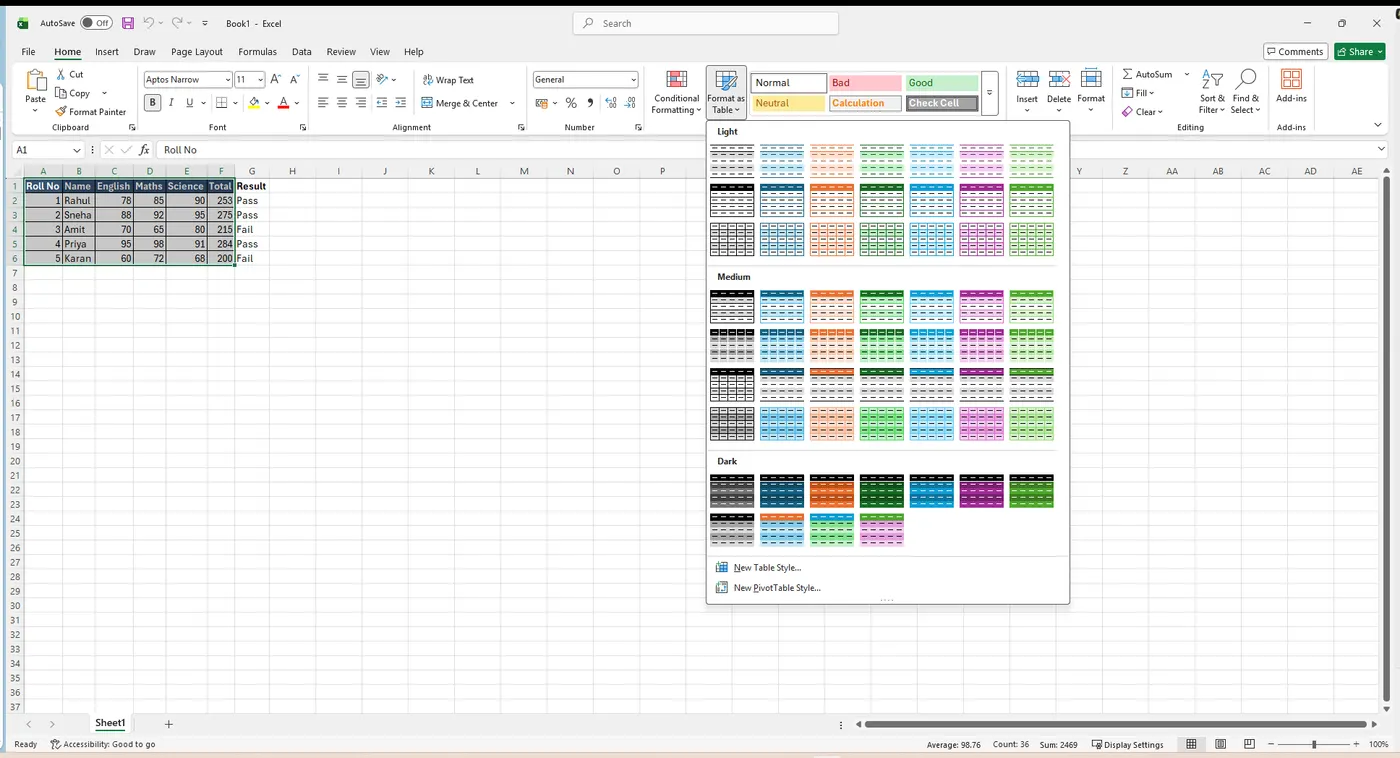
(1) Select the cells we want to format as a table. (2) From the Home tab, click the Format as Table command in the Styles group. (3) Select a table style from the drop-down menu. (4) A dialog box appears, confirming the selected cell range for the table. (5) If the table has headers, check the box next to My table has headers, then click OK. (6) The cell range is formatted in the selected table style.
Removing a table
Sometimes we may not want the additional features included with tables, such as the Sort and Filter drop-down arrows. We can remove a table from the workbook while still preserving its formatting elements, like font and cell colour. (a) Select any cell in the table — the Design tab appears. (b) Click the Convert to Range command in the Tools group. (c) A dialog box appears; click Yes. (d) The range is no longer a table, but the cells retain their data and formatting.
Charts
It can often be difficult to interpret Excel workbooks that contain a lot of data. A chart turns the workbook data into a picture, which makes it easy to visualise comparisons and trends. Excel has many different types of chart — Column, Bar, Line, Pie, Area and more — so we can choose the one that best fits our data; each chart type has its own advantages, so it helps to understand how different charts are used. We also need to understand how to read a chart: charts contain several different elements, or parts, that help us interpret the data.
Inserting a chart
(a) Select the cells we want to chart, including the column titles and row labels — these cells will be the source data. (b) From the Insert tab, click the desired Chart command. (c) Choose the desired chart type from the drop-down menu. (d) The selected chart is inserted in the worksheet. If we are not sure which type to use, the Recommended Charts command suggests several charts based on the source data.
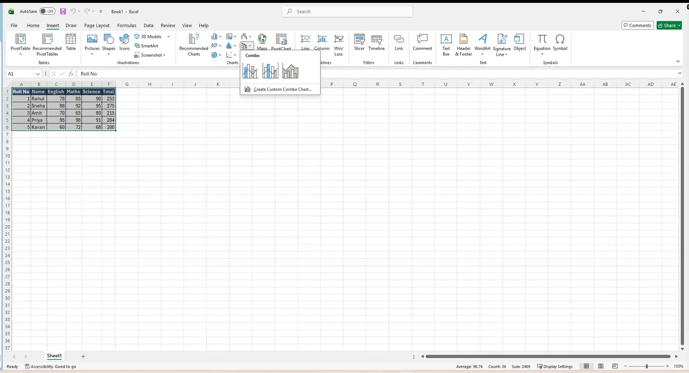
Chart layout & style
After inserting a chart, there are several things we might want to change about the way the data is displayed; it is easy to edit a chart's layout and style from the Design tab. Excel lets us add chart elements — such as chart titles, legends and data labels — to make the chart easier to read. To add one, click the Add Chart Element command on the Design tab and choose the desired element from the drop-down menu.
Comments & Conditional Formatting
Adding a comment
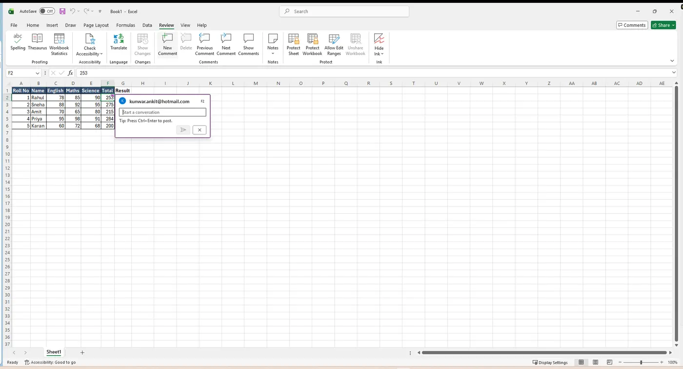
A comment is a little note attached to a cell. (a) Select the cell where we want the comment to appear — in our example, cell E8. (b) From the Review tab, click the New Comment command. (c) A comment box appears; type the comment, then click anywhere outside the box to close it. (d) The comment is added to the cell, represented by a red triangle in the top-right corner. (e) Select the cell again to view the comment. From the Review tab, the Show All Comments command displays every comment in the worksheet at the same time.
Conditional Formatting
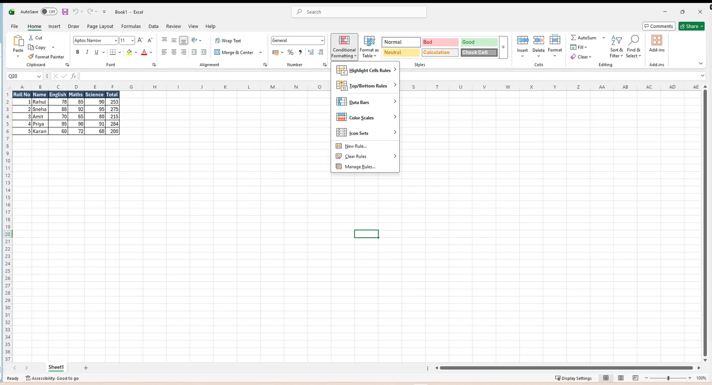
If we have a worksheet with thousands of rows of data, it would be extremely difficult to see patterns and trends just from examining the raw information. Similar to charts, conditional formatting provides another way to visualise data and make worksheets easier to understand. It automatically applies formatting — such as colours, icons and data bars — to one or more cells based on the cell value. To do this we create a conditional formatting rule. For example, a rule might be: “If the value is less than $2,000, colour the cell red.” By applying this rule we can quickly see which cells contain values under $2,000. To apply it:
(a) Select the desired cells for the rule. (b) From the Home tab, click the Conditional Formatting command — a drop-down menu appears. (c) Move the mouse over the desired formatting type (Highlight Cells, Data Bars, Colour Scales, Icon Sets, Top/Bottom Rules) and select the desired rule from the menu that appears. (d) A dialog box appears; enter the desired value(s) into the blank field. (e) Select a formatting style from the drop-down menu, then click OK. (f) The conditional formatting is applied to the selected cells.
Pivot Tables
When we have a lot of data, it can be difficult to analyse all of the information in a worksheet. PivotTables make worksheets more manageable by summarising data and allowing us to manipulate it in different ways. Suppose we wanted to answer the question: “What is the amount sold by each salesperson?” for some sales data. Answering this directly could be very time-consuming because each salesperson appears on multiple rows, and we would need to total all of their individual orders. We could use the Subtotal command to help, but we would still have a lot of data to work with. Fortunately, a PivotTable can instantly calculate and summarise the data in a way that is both easy to read and to manipulate. Once created, we can use it to answer different questions by rearranging — or pivoting — the data; for example, modifying it to answer “What is the total amount sold in each month?”.
To create a PivotTable: (a) select the table or cells (including the column headers) containing the data; (b) from the Insert tab, click the PivotTable command; (c) the Create PivotTable dialog box appears — choose the settings and click OK; (d) a blank PivotTable and Field List appear on a new worksheet; (e) decide which fields to add (each field is simply a column header from the source data) and check the box for each field in the PivotTable Field List; (f) the selected fields are added to one of the four areas below the Field List — Filters, Columns, Rows and Values; (g) the PivotTable calculates and summarises the selected fields. Drag fields between the four areas to pivot and see the data a new way.
What-If Analysis
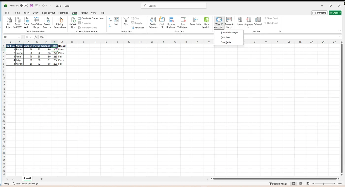
Excel includes many powerful tools to perform complex mathematical calculations, such as What-If Analysis (on the Data tab). This feature helps us experiment and answer “what would happen if…?” questions with our data, even when the data is incomplete. It offers three tools — Scenario Manager, Goal Seek and Data Table.
Open it Data → What-If Analysis shows Scenario Manager, Goal Seek and Data Table.
Goal Seek
Whenever we create a formula or function in Excel, we put various parts together to calculate a result. Goal Seek works in the opposite way: it lets us start with the desired result, and it calculates the input value that will give us that result. For example — “what must I score on the final assignment to reach 70 overall?”. To use it: (a) select the cell whose value we wish to change (this cell must already contain a formula or function); (b) from the Data tab, click What-If Analysis → Goal Seek; (c) a dialog box appears with three fields:
- Set cell — the cell that will contain the desired result (in our example, cell B7 is already selected).
- To value — the desired result (in our example, 70, because we need at least that to pass the class).
- By changing cell — the cell where Goal Seek will place its answer (in our example, cell B6, the grade we need on the final assignment).
(d) When done, click OK. (e) The dialog box tells us if Goal Seek was able to find a solution; click OK. (f) The result appears in the specified cell.
Other types of What-If Analysis
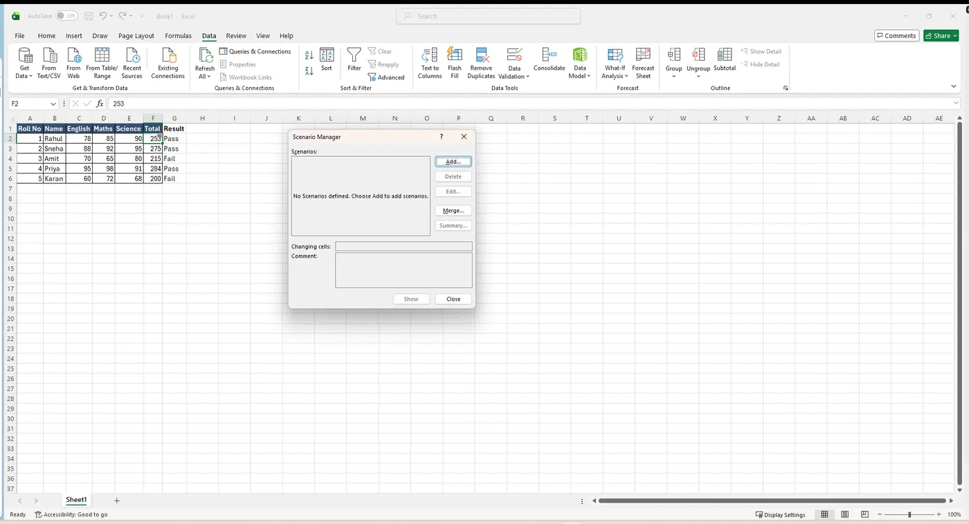
For more advanced projects we may consider the other two types — scenarios and data tables. Rather than starting from the desired result and working backward, like Goal Seek, these options let us test multiple values and see how the results change.
- Scenarios let us substitute values for multiple cells (up to 32) at the same time. We can create as many scenarios as we want and then compare them without changing the values manually. (Click the Add button to make a scenario.)
- Data Tables let us take one or two variables in a formula and replace them with as many different values as we want, then view the results in a table. This option is especially powerful because it shows multiple results at the same time — unlike scenarios or Goal Seek.
Beyond the Basics
These extra tools are not in the original syllabus but are well worth knowing — they make you much faster in real work.
Key Facts & Shortcuts
Numbers worth memorising
| Item | Value | Item | Value |
|---|---|---|---|
| Rows in a sheet | 10,48,576 | Columns in a sheet | 16,384 (A–XFD) |
| Max sheets in a workbook | 255 | Default font | Calibri, 11 |
| Workbook extension | .xlsx | Formula begins with | = (equals) |
| Orientations | Portrait, Landscape | Currency format | Accounting |
Keyboard shortcuts
| Keys | Action | Keys | Action |
|---|---|---|---|
| Ctrl + N | New workbook | Ctrl + O | Open |
| Ctrl + S | Save | F12 | Save As |
| Ctrl + P | Ctrl + 1 | Format Cells | |
| Ctrl + B / I / U | Bold / Italic / Underline | Ctrl + Z / Y | Undo / Redo |
| Ctrl + C / X / V | Copy / Cut / Paste | Ctrl + F / H | Find / Replace |
| Shift + F3 | Insert Function | F4 | $ absolute reference |
| Ctrl + Home | Go to A1 | Ctrl + E | Flash Fill |
Exam Question Bank
Objective questions frequently asked in GCC-TBC and Excel exams. Revise with the answer beside each.
| # | Question | Answer |
|---|---|---|
| 1 | To select a whole row, click on the ___. | Row number |
| 2 | The ___ function gives the minimum value in a range. | =MIN() |
| 3 | If you increase the height of a row, the text shifts to the ___ of the cell. | Bottom |
| 4 | Underline is used to make the text ___ in the selected cells. | Underlined |
| 5 | The ___ function inserts the current system time into the cell. | =NOW() |
| 6 | Cell addresses used in a formula are called ___. | Cell References |
| 7 | The ___ command joins two or more cells and centres the data. | Merge & Center |
| 8 | The ___ function counts how many cells in a range contain numbers. | =COUNT() |
| 9 | A function always starts with the ___ symbol. | = (equals) |
| 10 | To make a graph from data, the ___ command is used (Insert tab). | Charts |
| 11 | The option to increase the font is available in the ___. | Font group |
| 12 | A single worksheet has ___ rows. | 10,48,576 |
| 13 | The bar that shows the content and formula of the active cell is the ___ Bar. | Formula |
| 14 | A workbook can have a maximum of 255 ___. | Sheets |
| 15 | To apply Currency style, use the ___ option in the Number group. | Accounting Number Format |
| 16 | How many orientation types are available in MS Excel? | Two |
| 17 | The file extension .xlsx means ___. | Microsoft Excel Workbook |
| 18 | You cannot use ___ while typing a formula in a cell. | Spaces |
| 19 | The AutoSum option is available in the ___ tab. | Formulas |
| 20 | A data Filter is used when a table is ready in the ___. | Worksheet |
| 21 | To delete only the data but keep the format, use ___. | Clear Contents |
| 22 | Which alignments are available in Excel? | All of the above |
| 23 | Pressing the Home key moves the cell pointer to the first cell of the current row. | True |
| 24 | A collection of worksheets is called a ___. | Workbook |
| 25 | ___ means an instruction to perform a calculation. | Formula |
Exam Question Bank (cont.)
| # | Question | Answer |
|---|---|---|
| 26 | Only a graph is shown in a ___ sheet. | Chart |
| 27 | The Sort and Filter commands of the Home tab are also on the ___ tab. | Data |
| 28 | ___ means a built-in formula available in Excel. | Functions |
| 29 | The =TODAY() function gives the current ___. | Date |
| 30 | The ___ feature shows the total of selected cell values on the status bar. | Sum |
| 31 | The ___ option is used to rotate text in a cell. | Text Orientation |
| 32 | The heading of the last column in a worksheet is ___. | XFD |
| 33 | Pressing the ___ key moves the cell pointer to the first cell of the current row. | Home |
| 34 | MS Excel is a ___ type of application software. | Spreadsheet |
| 35 | In MS Excel, a Hard Copy is the ___ of a file. | Printed copy |
| 36 | To remove the Freeze effect, choose ___ (View → Window → Freeze Panes). | Unfreeze Panes |
| 37 | The ___ option shows rows based on a specific condition. | Filter |
| 38 | The ___ command is used to open a new sheet. | New |
| 39 | The =MAX() function is used to find the ___ number. | Largest |
| 40 | Ascending sorting means ___ sorting. | A to Z |
| 41 | Cell references that change automatically when a formula is copied are called ___. | Relative References |
| 42 | Portrait and Landscape are types of ___. | Orientation |
| 43 | Cell references that stay the same when a formula is copied are called ___. | Absolute References |
| 44 | =SUM(F8:F12) sorts the values in the range F8 to F12. | False |
| 45 | To select the whole sheet, use the ___ key combination. | Ctrl + A |
| 46 | Page breaks are viewed in ___. | Page Break Preview |
| 47 | Scroll bars are used to view different areas of the worksheet. | True |
| 48 | Format Painter is available in MS Excel. | True |
| 49 | A-to-Z serial means ___ sorting of text. | Ascending |
| 50 | The selected single cell in a worksheet is called the ___. | Active Cell |
Exam Question Bank (cont.)
| # | Question | Answer |
|---|---|---|
| 51 | The arrow keys (navigation keys) move the cell pointer one cell at a time. | True |
| 52 | In a workbook, the default sheet names are displayed on the ___. | Sheet Tab |
| 53 | Pictures can be inserted from the ___ tab. | Insert |
| 54 | Ctrl + Page Down can be used to go to the next sheet. | True |
| 55 | Cell alignment in Excel is done from ___. | Home → Alignment |
| 56 | The options to change font size, colour and face are in the ___. | Font group |
| 57 | Gridlines have vertical and horizontal lines. | True |
| 58 | Cell references can be made absolute using the ___ symbol. | $ |
| 59 | IF is not a logical function. | False |
| 60 | The date format in a cell is ___. | MM-DD-YY |
| 61 | To start Excel, click the ___ button on the taskbar. | Start |
| 62 | The height of a row is measured in which unit? | Point |
| 63 | The two types of sorting in Excel are ___. | Ascending & Descending |
| 64 | The Top/Bottom Rules of Conditional Formatting can be used only for ___. | Numeric Data |
| 65 | Using the Exit option does what in Excel? | Quits Excel |
| 66 | The active cell is recognised by a ___ around it. | Black border |
| 67 | To select a complete row, click on the ___. | Row Number |
| 68 | MS Excel creates a ___ type of file. | Workbook |
| 69 | The ___ function rounds a number to a specific number of digits. | =ROUND() |
| 70 | The ___ tool inserts readymade shapes like Rectangle, Arrow and Line. | Insert → Shapes |
| 71 | It is not possible to insert a column in the work area. | False |
| 72 | To select a range, use the arrow keys with the ___ key. | Shift |
| 73 | A typed cell value is displayed in the ___. | Formula Bar |
| 74 | Where a row and a column intersect (a square) is called a ___. | Cell |
| 75 | At the left side of the Zoom Slider we see the ___. | Status Bar |
Exam Question Bank (cont.)
| # | Question | Answer |
|---|---|---|
| 76 | A formula is an instruction to perform a ___. | Calculation |
| 77 | DB is a financial function. | True |
| 78 | A new comment can be inserted from the ___ tab. | Review |
| 79 | The =UPPER() function converts the given text into ___. | Capital letters |
| 80 | When you copy a formula, Excel erases the original copy of the formula. | False |
| 81 | Z-to-A serial means ___ sorting of text. | Descending |
| 82 | The Help option is available in the ___ menu. | File |
| 83 | After starting MS Excel, the default file we see is ___. | Book1 |
| 84 | ___ is present by default in Excel. | Gridlines |
| 85 | A workbook can have a maximum of ___ sheets. | 255 |
| 86 | Descending sorting means ___ sorting. | Z to A |
| 87 | The shortcut key for closing an Excel workbook is ___. | Ctrl + W |
| 88 | ___ is used to insert artistic graphics to communicate information visually. | SmartArt |
| 89 | The Recent option is available in the ___ menu. | File |
| 90 | Delete Sheet command is given in the ___ tab (Cells group). | Home |
| 91 | ___ is NOT a type of view in Excel. | Print Layout |
| 92 | The strip to the right of the Name Box is called the ___ Bar. | Formula |
| 93 | Each Excel file is called a workbook because ___. | it can contain many sheets |
| 94 | We cannot use ___ alignment in Excel. | Justify |
| 95 | A symbol can be inserted using the ___ menu. | Insert |
| 96 | The Zoom option is available on the ___ tab. | View |
| 97 | The syntax of the IF function is =IF(Condition, value if True, value if False). | True |
| 98 | A Pivot Table is used to ___. | Summarise data |
| 99 | A ___ is used for different mathematical calculations in Excel. | Formula |
Chapter Mind Map
One-glance revision of the whole chapter — follow each branch to recall the key points.
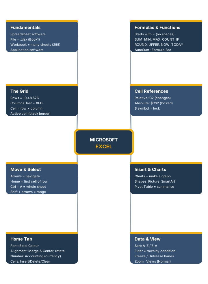
Image Credits & Notes
All screenshots in this book were captured first-hand in Microsoft Excel on a clean sample marksheet created for teaching. They contain no personal data. Screenshots are used to illustrate Microsoft Excel's interface for educational purposes; Microsoft Excel is a product of Microsoft Corporation.
The GradeTyping logo, page layout, diagrams and the chapter mind map are original GradeTyping artwork (vector SVG).